How to Split Data Into Multiple Columns in Excel

Splitting the contents of a cell into more than one column manually in Microsoft Excel would take too much time and likely result in errors. Fortunately, the program offers many ways—from built-in tools and automated processes to easy-to-use functions—to execute this data-sorting task.

Using the Text to Columns Tool

One way to split data into multiple columns in Microsoft Excel is to use the built-in Text To Columns tool. This method is handy if you prefer to work in a dialog box that guides you through the process.

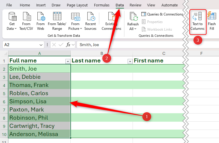
For example, let’s say you want to split the names in column A into last and first names in columns B and C, respectively.

To do this, first, select the cells in column A, and in the Data tab on the ribbon, click “Text To Columns.”

In the Convert Text to Columns Wizard, select “Delimited,” and click “Next.”

A delimiter is a character, symbol, or space that is used to separate items in a sequence. In this example, the names in column A are separated by a comma and a space, so check both these options. You can see how this will affect your data in the preview at the bottom of the dialog box. If you’re happy, click “Next.”

Next, clear any information in the Destination field, select the cell where you want the split data to be—in this case, cell B2—and click “Finish.”

Now, the full names are split into last and first names in their respective columns. If needed, you can delete the original data in column A, as the split names aren’t linked in any way to the full names.

However, in this example, one person has two first names, and another person has two surnames. In this case, selecting the space delimiter will split these dual names into separate columns, even though you want to keep them together.

To overcome this, select the comma delimiter only—not the space delimiter—in the Convert Text to Columns Wizard.

Once the splitting process is complete, however, you’ll notice that the first names are preceded by a space, as you didn’t tell Excel to consider spaces as delimiters.

To remove these spaces, expand the table one column to the right to create another column for the corrected first names. Then, in cell D2, type:

=TRIM((@(First name)))

where the TRIM function removes all spaces from a text string (except for spaces between words), and (@(First name)) is a structured reference to the column in the table called “First names.”

Related

How to Use the TRIM Function in Microsoft Excel

Remove unnecessary white spaces from text strings.

When you press Enter, the first names will appear in column D, but this time, without the leading space. Also, because the data is in a formatted Excel table, the formula is duplicated automatically in the remaining cells of the column.

Next, select the newly generated first names, and press Ctrl+C to copy them. Now, press Ctrl+Alt+V to open the Paste Special dialog box, then V to select “Values,” then Enter.

Finally, delete the column containing the spaces before the first names (C) and the original column containing the full names (A) to complete your table.

Microsoft Excel has many tools to automate otherwise tedious processes, and Flash Fill is one of the most useful.

If using the Text To Columns Wizard to split data into more than one column takes too much time, this intuitive tool will help speed things up. In essence, it’s a smarter way to copy and paste the data into new cells.

Related

Short On Time? Use These Excel Tips to Speed Up Your Work

Use Excel’s time-saving tools to get jobs done.

First, select the cell where you want the first split element to go (in this case, cell B2), type the value (in this case, Smith) manually, and press Enter.

Next, in the Data tab on the ribbon, click “Flash Fill.”

When you run Flash Fill, Excel looks for patterns in the data, and tries to apply them to the remaining data in the range. In this example, it successfully fills in the rest of the last names from the original data down column B.

Then, repeat the process for the first names in column C—type the first value to set the pattern, press Enter, then press Ctrl+E.

Using Built-In Excel Functions

Another way to split data into multiple columns is to use some of Microsoft Excel’s functions. If you choose this route, remember that the split values will be linked to the original values, meaning you need to copy (Ctrl+C) and paste them as values (Ctrl+Alt+V > V) if you want to delete the original data.

TEXTSPLIT

Excel’s TEXTSPLIT divides all content in a cell into different columns according to a delimiter you specify, and returns the result as a spilled array.

Related

Everything You Need to Know About Spill in Excel

It’s not worth crying over spilled references.

In this example, let’s assume you want to split the capitals and states in column A into columns B and C using a single formula.

To do this using TEXTSPLIT, in cell B1, type:

=TEXTSPLIT(A2,", ")

where A2 is the cell containing the text you want to split, and the comma + space combination wrapped in quotation marks tells Excel that these characters together form the delimiter.

When you press Enter and select the cell where you just typed the formula, you’ll see a blue line surrounding the result. This means that even though you only typed the formula into cell B2, the result has spilled over into cell C2.

Because the data is in a range that isn’t formatted as an Excel table, you need to fill the rest of the column manually. To do this, click and drag the fill handle in the bottom-right corner of cell B2 to the bottom of the range.

TEXTBEFORE and TEXTAFTER

Where TEXTSPLIT divides all the contents of a cell, the TEXTBEFORE and TEXTAFTER functions let you choose whether you want to extract the information before or after a delimiter. Also, as they’re not dynamic array functions, you can use them in data formatted as a table.

Using the same example as above, starting with the state capitals, in cell B2, type:

=TEXTBEFORE((@(Capital and State)),", ")

where (@(Capital and State)) is a structured reference to the column containing the cells you want to split, and the comma + space combination inside quotation marks tells Excel that a comma followed by a space should be considered as the delimiter. This time, however, only the text before the delimiter is returned in the result when you press Enter.

Related

Everything You Need to Know About Structured References in Excel

Use table and column names instead of cell references.

So, to extract the last names in cell C2, type:

=TEXTAFTER((@(Capital and State)),", ")

and press Enter.

Alongside their compatibility with Excel tables, a benefit of using TEXTBEFORE and TEXTAFTER instead of TEXTSPLIT is that the results don’t need to be in adjacent columns.

LEFT, MID, and RIGHT

Excel’s LEFT, MID, and RIGHT functions allow you to split a cell’s content at certain positions within the character string. This is particularly handy if you have a dataset of structurally consistent values, like a serial number or a code.

Related

How to Extract a Substring in Microsoft Excel

Get the important part while leaving the rest out!

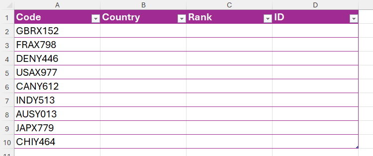
In this example, the first three characters represent a country, the last three characters represent an ID, and the X or Y in the middle represent a rank. Your aim is to split these three elements into columns B, C, and D, respectively.

First, to extract the countries, in cell B2, type:

=LEFT((@Code),3)

where LEFT((@Code) tells Excel to read cells in the Code column from the left, and 3 tells Excel to extract the first three characters.

Now, in cell D2, follow the same principle, but use the RIGHT function to extract the last three characters:

=RIGHT((@Code),3)

Finally, in cell C2, you want to extract the middle character, which is the fourth in the string. To do this, type:

=MID((@Code),4,1)

where 4 tells Excel to begin the extraction from the fourth character, and 1 tells Excel that you only want to extract a single character.

Now, you’ve successfully split the data in column A into three separate columns.

Using the Power Query Editor

Many people believe that Excel’s Power Query Editor is too complex for them—however, it was designed specifically to be user-friendly and is a great way to split data into multiple columns.

In this example, let’s say you have this Excel table containing various NFL teams, and you want to split these into their respective regions and team names.

First, select any cell in the data, and in the Data tab on the ribbon, click “From Table/Range” in the Get And Transform Data group.

This launches the Power Query Editor, which is where the magic happens!

Right-click the header of the column you want to split, and click Split Column > By Delimited.

Then, in the dialog box, choose the delimiter—in this case, it’s a space—and review the data to work out at which delimiters you want the data to be split. Since some regions in NFL team names have more than one word, but all their suffixes contain only one word, the text needs to be divided by the right-most delimiter.

Now, when you click “OK,” you’ll see the team names divided into two columns at the final delimiter. At this point, double-click the new column headers to rename them.

Finally, click the top half of the “Close And Load” icon in the top-left corner of the Power Query Editor, and the newly split data will open in a new worksheet.

Related

How to Clean Up and Import Data Using Power Query in Excel

Don’t overlook this amazing Excel tool!

Splitting data into multiple columns isn’t the only way to rearrange data in Excel. For example, you could merge data from two columns into one column, split alternate rows into two columns, or turn vertical data horizontal. Regardless of how you want to organize your data, there’s likely a built-in Excel tool that will help you along your way.